

Tools Used: Hill Climb Search, Discrete Bayesian Networks, Hidden Markov Models, Permutation Testing, Combinatorial Purged Cross Validation, Backtesting, Probabilistic Sharpe Ratio, Deflated Sharpe Ratio, fredapi, matplotlib, networkx, numpy, pandas, pgmpy, pomegranate, scipy, seaborn, sklearn, yfinance
Project GitHub Link
Project HTML Link
Motivation
In one of my Master’s degree courses, I read an interesting Bachelor’s thesis paper titled, “Application of Probabilistic Graphical Models in Forecasting Crude Oil Price.” It was written in 2018 by a student named Danish Alvi. In the paper, Alvi tried to predict the price of oil futures one month ahead using Hidden Markov Models and Bayesian Networks. The author found some evidence that this approach might be able to capture monthly patterns in the data.
Fascinated by the core idea, I decided to do something similar here but with the goal of predicting price movements on a five-day horizon rather than a one-month horizon. I suspected this might be a more challenging task, since market patterns that exist on a monthly timeframe tend to devolve into noise on shorter timeframes. My hope was that this might provide more convincing evidence, given the greater quantities of daily price data that are available and my desire to improve upon the analysis methods used in the original paper.
Overview
With that motivation, this project will explore how to:
- Identify market regimes using a Hidden Markov Model.
- Construct and fit the parameters for a Bayesian Network.
- Use a Bayesian Network to inform trading decisions on front-month oil futures.
All of the code for this project, along with the results and some of the analysis, can be found in the Jupyter Notebook on my GitHub under “ryancardenas/demos/finance/Predicting Oil Price Action”. Just in case GitHub doesn’t render the notebook, it can also be viewed directly on this website.
Let’s dive right in!
Step 1: Define performance metrics.
Classification Performance
Before we begin building and evaluating the model, we should determine how we want to measure its performance. Ultimately, our goal is to predict whether WTI Oil front-month futures (shown as “CL=F” on Yahoo Finance) will increase or decrease in price over the next 5 trading days. Since there are only two possible outcomes, this is a binary classification problem. We will want to measure:
- Accuracy as our primary metric, because a long-and-short strategy will depend heavily on our overall rate of correct guesses. This should be greater than 50%, hopefully by a wide margin.
- Precision, because a long-only strategy will depend heavily on how many of our “increase” guesses are correct.
- Recall, because an analyst using a long-only strategy might be interested in how many opportunities they missed.
- F1-score, because it combines precision and recall in a balanced way.
We will use SciPy’s implementation of these functions.
Statistical Significance
Additionally, for any set of data that we try to predict, we want to know the answer to this question:
- What are the chances our model achieved its accuracy purely by luck, rather than by identifying a legitimate pattern in the market?
To answer this question, we can use a permutation test where we simulate a bunch of random scenarios with the same proportions of answers as our data, but shuffled around, and then compare our model’s predictions in the real world against the simulated random worlds. It’s kind of like asking, “Out of 100,000 worlds where oil prices do not follow any intelligible pattern, in how many of those worlds would our model have achieved an equal or greater accuracy than what we found in the real world?” If the answer to that question is a very small number, then it’s likely that oil prices in the real world do follow a pattern and that our model captured it.
Impact on Trading
Since we aim to build a model that provides a reliable trading signal, we will compare the metrics for three different strategies:
- A baseline buy-and-hold strategy on CL=F. The idea is to allocate 100% of the portfolio to CL=F futures with a single trade at the beginning and rollover the position with zero extra costs a few days before the end of each month. This portfolio will follow the price of WTI Oil futures.
- A model-informed long-only strategy where we go long whenever the Bayesian Network predicts a positive price movement over the next five days, do nothing whenever a negative price movement is predicted, and exit open positions at the close of day exactly five days after the entry.
- A model-informed long-short strategy, where we go long with positive predictions and short with negative predictions, hoping to capture the full range of price movements.
For each of these three strategies, we will compute the following metrics:
- Final profit and loss as a ratio. We want this to be a large number.
- Max drawdown as a ratio. We want this to be a very, very small number…
- Calmar Ratio, which measures compound annual growth rate in excess of risk-free returns divided by the max drawdown. This allows us to compare the portfolio’s gains to its largest loss.
- Omega Ratio, which compares the probability-weighted returns for winning trades (in excess of the de-annualized risk-free rate) to the probability-weighted returns for losing trades. This provides a different measure of reward versus risk than the Calmar Ratio.
- Sharpe Ratio, which compares the average excess return to the standard deviation of excess returns. There are many problems with the Sharpe Ratio since it makes some assumptions that definitely aren’t true, but it’s widely used nonetheless.
- Probabilistic Sharpe Ratio, which computes the probability that our strategy’s true Sharpe Ratio exceeds that of the benchmark buy-and-hold strategy. This is useful for sanity-checking our measured Sharpe Ratio. We will aim for a PSR > 0.95 to dismiss the null hypothesis of not exceeding the benchmark.
- Deflated Sharpe Ratio, which computes the probability that our strategy’s true Sharpe Ratio exceeds the largest Sharpe Ratio we would expect to see from testing multiple random strategies. The more strategies we test, the easier it is to find one with a high Sharpe Ratio purely by chance, and the easier it is to fool ourselves into thinking we struck gold when all we really did is draw too many strategies out of a hat. This metric helps us to avoid that. We’re looking for DSR > 0.95 to dismiss the null hypothesis of not exceeding the random noise Sharpe Ratio.
Step 2: Run ETL pipeline.
Extract
We don’t necessarily know ahead of time what information will be useful for predicting the price of oil futures, but some viable candidates are stocks of oil companies, an energy sector index or exchange-traded fund (ETF), a general market index/ETF, and macroeconomic or energy-related data published by the federal government.
We will source daily market data for futures, stocks, ETFs, and indices using the yfinance module in Python, which interfaces with Yahoo Finance’s API. For the economic and energy data, we will use the Federal Reserve Economic Data (FRED) and U.S. Energy Information Administration (EIA) APIs to access publicly available government databases. Since we want as much data as possible for training our model, we will download all available data for each of the features shown in Table 2.1 below.
| Symbol | Description | Source | Sampling Frequency | Availability Lag [days] |
|---|---|---|---|---|
| ^SPX | S&P 500 general market index | Yahoo Finance | daily | 1 |
| BZ=F | Brent Crude Oil front month futures price | Yahoo Finance | daily | 1 |
| CL=F | West Texas Intermediate (WTI) Oil front month futures price | Yahoo Finance | daily | 1 |
| CVX | Chevron stock price | Yahoo Finance | daily | 1 |
| SHEL | Shell PLC stock price | Yahoo Finance | daily | 1 |
| XLE | S&P 500: Energy Sector exchange-traded fund (ETF) price | Yahoo Finance | daily | 1 |
| XOM | Exxon Mobile stock price | Yahoo Finance | daily | 1 |
| A24ATI | Manufacturers’ Total Inventories: Petroleum Refineries | FRED | monthly | 65 |
| CAPG211S | Industrial Capacity: Mining: Oil and Gas Extraction | FRED | monthly | 65 |
| CAPUTLG211S | Capacity Utilization: Mining: Oil and Gas Extraction | FRED | monthly | 65 |
| CPIENGSL | Consumer Price Index for All Urban Consumers: Energy in U.S. City Average | FRED | monthly | 65 |
| IPG21112S | Industrial Production: Mining: Crude Oil | FRED | monthly | 65 |
| IPN213111N | Industrial Production: Mining: Drilling Oil and Gas Wells | FRED | monthly | 65 |
| INDPRO | Industrial Production: Total Index | FRED | monthly | 65 |
| OVXCLS | CBOE Crude Oil ETF Volatility Index | FRED | daily | 2 |
| PCU211211 | Producer Price Index by Industry: Oil and Gas Extraction | FRED | monthly | 65 |
| WTISPLC | Spot Crude Oil Price: West Texas Intermediate. Even though we already have CL=F in our list of features, we include this because it allows us to track month-to-month changes that are also from a different source. | FRED | monthly | 65 |
| PAPR_OPEC | Total OPEC Petroleum Supply (million barrels per day) | EIA | monthly | -453 |
| RCRR01NUS_1 | U.S. Crude Oil Proved Reserves (Million Barrels) – up to 2023 | EIA | annually | 1707 |
| RCRR01R48F_1 | U.S. Federal Offshore Crude Oil Proved Reserves (Million Barrels) – up to 2023 | EIA | annually | 1707 |
| WGFUPUS2 | U.S. Product Supplied of Finished Motor Gasoline (Thousand Barrels per Day) | EIA | weekly | 13 |
Transform
To predict price changes in the near future, we will want to first transform our data into percent changes:
$$\Delta_{pct}=\frac{p_{t+1}-p_t}{p_t}$$
After computing percent changes, we will merge all times series onto a common timeline. Most of the economic data is sampled on a monthly or annual basis whereas the stock data is sampled daily, so we will forward fill all series onto the datetime index of CL=F before merging. This approach represents the fact that, at any point in time, we will always have access to historical data from earlier in the timeline.
The big caveat is that data generally becomes available after a lag period. For instance, we won’t know the daily closing price of a stock until after the market closes, and we won’t be able to make a trading decision based on that information until the next day. Similarly, much of the economic and energy data becomes available only after the government agencies have completed their official data collection processes and reports. FRED data can take 1-2 months to publish; EIA data often becomes available 2-3 years after the fact. Fortunately, we can measure the lag periods for each feature by counting the days between now and the most recent datum, as shown in the last column of Table 2.1. Once we have measured the lag for each feature, we should round up to the nearest whole unit of the sampling frequency to make sure we don’t bias our estimated lag with the date of our data extraction. For example, we can round a 65-day lag on monthly data up to 3 months; we can round a 13-day lag on weekly data up to 2 weeks.
Once we have our estimated lag for each feature, we will then shift each feature’s time series forward by that number of periods to represent the fact that, at any point in time, we only have access to historical data that has already been published. A monthly economic measurement posted for January 1st, 2025 with a 2-month publishing lag will be shifted to roughly March 1st, 2025 (“roughly” because we will assume that months are 30-days long for the purposes of shifting data), since that is the soonest we would have had access to that data. This will eliminate any look-ahead bias in our data; we still have to do some work to prevent look-ahead bias in our models, but that will come later.
The entire cleaning and transforming pipeline follows this process:
- Compute the 5-day percent change of CL=F. This is our target feature, the direction of which we will try to predict.
- Handle lags in data availability by shifting each time series forward in time according to its respective lag.
- Assume that years have 365 days, months have 30 days, and weeks have 7 days.
- Let the
pandasmodule handle the shifting logic based on the sampling frequency of each time series.
- Compute the single-period (in contrast with the target’s 5-period horizon) percent changes of all other features in their respective sampling frequencies. For daily sampled data, this will be daily percent changes; for monthly data, it will be monthly percent changes, and so forth.
- Resample all features onto the daily timeline index of CL=F.
- Forward fill any gaps to reflect the fact that we still have access to the data that came before.
- Merge all features into a single DataFrame, including the target feature.
- Remove any rows containing duplicate indices so that we don’t over-train our models on any single datum.
- Forward fill any gaps in the merged DataFrame, as an extra precaution.
- Drop any rows containing missing values. At this point, the only rows with missing values should be at the start of the timeline, since some of the time series have data going back to the 1920s while others only go back to the 2000s.
- Drop any rows representing dates after the LAST_ANALYSIS_DATE, which is set to “2025-09-01” for repeatability. This is particularly important for the EIA Short Term Energy Outlook data, which forecasts multiple years into the future. In real life, we would have access to these predicted values years before their posted dates elapse, so truncating them is a conservative approach that will prevent any missing “future data” for features that aren’t forecasts.
Load (Train/Val/Test Split)
Once we have extracted and transformed our data, we will partition it into Training, Validation, and Testing sets. The purpose of the Training set is to tune the parameters of our model to fit the data. The purpose of our Validation set is to tune the hyperparameters of our model development process — a metacognitive task that allows us to validate our architectural assumptions and evaluate model performance out-of-sample. Once we have finalized our hyperparameters, we will retrain the model on the combined Training-Validation data and conduct a final assessment of the model’s predictive ability using the Testing set. The sole purpose of the Testing set is to pass or fail our final model.
We want enough Training data for the model to learn any lasting patterns that may exist in the market, but we also want enough Validation and Testing data to reliably evaluate how the model performs on new data. Since we’re dealing with daily price action, 2-3 years of data should be enough for computing statistical moments. We will split the cleaned data according to Table 2.2 below:
| Set | Start Date | End Date | # Data Points |
|---|---|---|---|
| TRAIN | 2007-08-01 | 2018-12-31 | 2875 |
| VAL | 2019-01-02 | 2022-12-30 | 1008 |
| TEST | 2023-01-03 | 2025-08-29 | 670 |
It’s worth stating explicitly that we want to minimize the number of times we change our hyperparameters after viewing the Validation set. The reason for this is that every time we change something based on the Validation set — either in the model or in our way of approaching the problem — information leaks from the Validation set into the training of our model. At some extreme point, we will have ended up fitting our model to the Validation set if we’re not careful. That’s fine if we are retraining the model in preparation for its final evaluation on the Testing set, but it’s counterproductive if we are trying to identify the best approach to solving a problem, because we can’t validate our approach if we have been peaking at the answers too often.
That’s also why we will only use the Testing set at the very end, to evaluate the final model: we don’t want any information from the Test set to leak into the training of the model, accept that which involves accepting or rejecting the model for use in live trading.
Step 3: Conduct exploratory data analysis on Train.
Before trying to develop a model, it’s helpful to understand the training data. We will look for anything the stands out as unusual or significant, because it might reveal a bug in our process so far, or potentially a useful pattern. Upon finding that our data is well-defined, finite, and appropriately signed (it turns out that futures prices can, in fact, be negative! — more on this later…), we can look at a pairplot to visualize how the features are related to each other.
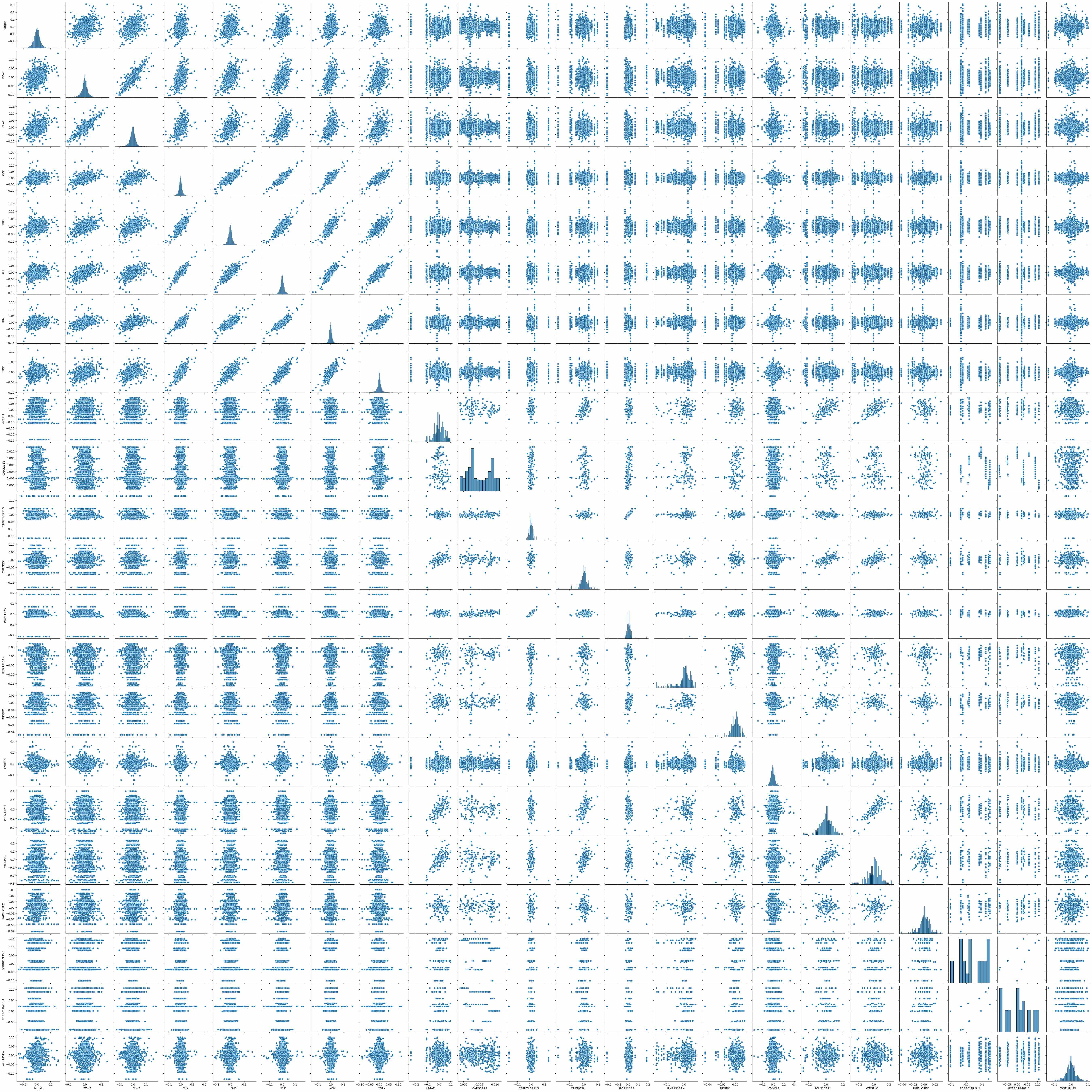
Figure 3.1 shows the “pairplot” of all 22 features. It’s essentially a grid of scatter plots comparing every feature against ever other feature, with histograms along the diagonal. Glancing at it, we can see that stocks, ETFs, and indices appear to vary linearly with one another. Most of the features are distributed continuously, with CAPG211S distributed bimodally and both of the reserves-oriented features distributed sparsely. Changes in proved oil reserves appear to take on a small set of discrete values, while the stock prices tend to have more continuously distributed price changes. This makes sense because the stock prices were sampled on a daily basis, whereas the proved oil reserves are sampled once per year and therefore have fewer unique data points. Most of the economic data appears to be non-normal, although looks can be deceiving and we would need to run proper normality tests to be sure. All of the scatter plots appear to be either uncorrelated or monotonically correlated, so we can look at a correlation heatmap for a different vantage point.
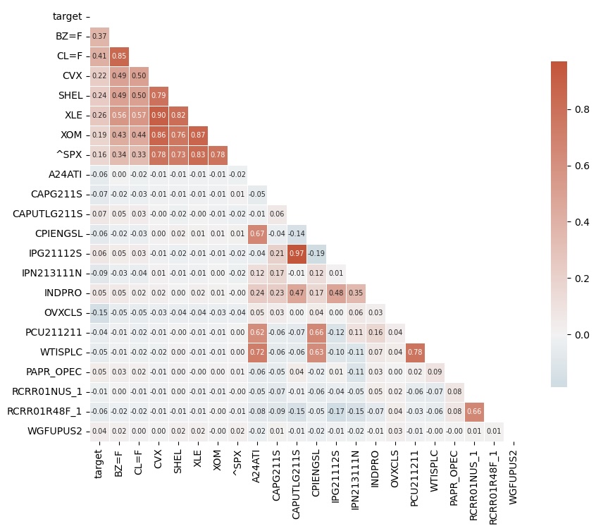
Figure 3.2 shows a heatmap of correlations. As expected, the stocks CVX and SHEL, along with the sector ETFs XLE and XOM all exhibit strong correlation with the general market index ^SPX, but more moderate correlation with oil futures BZ=F and CL=F. Meanwhile, the futures have strong correlation with each other. Oil/gas capacity utilization (CAPUTLG211S) and oil production (IPG21112S) are almost perfectly correlated, suggesting that we should examine the possibility of dropping one of them.
Closer Look: Utilization and Production
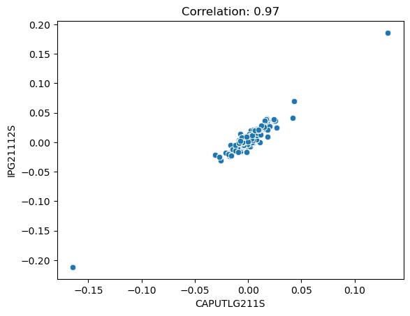
Taking a closer look at the scatter plot of capacity utilization versus oil production (Figure 3.3), we can see that most of the points are bundled closely together at the center of the plot. There appear to be two extrema that may be skewing the correlation, so let’s see what happens when we remove those points.
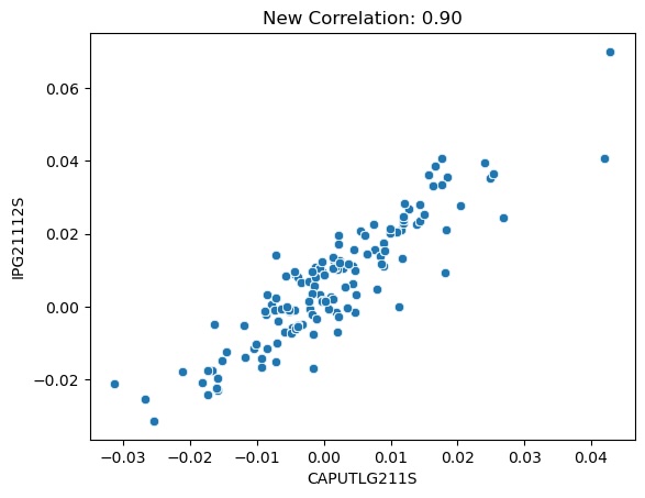
Figure 3.4 shows us that, even without the extrema, the data is still highly correlated with a Pearson coefficient of 0.90. Removing the extrema helped to lower the correlation noticeably, but not enough make either feature irreplaceable. It turns out that the points we removed belonged to 2008-12 and 2009-01. Remembering that we shifted these features forward 3 months, the picture becomes clearer: the extreme values came from September and October 2008, the two worst months of the 2008 market crash. Those were extraordinary times, so this economic data appears to be a realistic and fair representation of what happened. For that reason, we will not remove these outliers from the data. Since the capacity utilization (CAPUTLG211S) also reflects natural gas, it does technically introduce additional data not visible in oil production (IPG21112S), which is likely the reason for the less-than perfect correlation. We could probably drop one of these series without trouble, but on the off-chance the non-mutual information is useful, we will keep them both and let the model decide which one is more important.
Step 4: Build model development pipeline.
Combinatorial Purged Cross Validation
To improve our model development process and avoid overfitting our validation set, we will use combinatorial cross validation within our training set. To make sure our process is capable of predicting out-of-sample market dynamics for multiple years at a time, we will aim for segments of roughly 1 year each. Our training set spans 11.5 years, so we will divide it into 11 segments and choose 8 for training, with the remaining 3 for cross-validation. In every iteration, the model development process will train a model on ~8 years of data and predict on the unseen 3 years. This arrangement will give us 165 combinations, which is certainly enough to estimate the first and second statistical moments of our performance metrics.
$${\text{11 segments} \choose \text{8 for training}}=\text{165 combinations}$$
It is worth noting that each segment will occur in \({{n-1} \choose {k-1}}\) of the combinations, so we would expect to see the first segment appear in 120 out of 165 combinations given n=11 and k=8.
In cases where the last date in the CPCV training set occurs close to the first date in the CPCV validation set, the target variable will cause information to leak from the validation to the training set because it provides information about prices five days ahead of time. To avoid this, we will purge the last 5 days from every CPCV training set — a total of 40 days purged over the course of 8 training segments.
While we build our model development pipeline, we will use just one of the 165 CPCV groups for debugging. Then, when we have verified that everything runs smoothly, we will apply the pipeline to the entire CPCV set.
Data Discretization
Before we can use Hidden Markov Models to detect regime changes, we will want to discretize our continuous data. We will do this by replacing each value — which currently represents a continuous first derivative — with its sign. Positive price changes will be represented as a “1” and all other price changes as a “0”. While HMMs can be fashioned to handle continuous data, that can get messy when the distributional forms are not known. We don’t know which distributional forms best describe each feature, so discretizing by sign allows us to simplify our development process greatly.
Encoding Market Regimes
Labeling market regimes is challenging because there is no single “right answer.” Our goal is train an HMM that can identify when markets are generally trending upward, downward, or sideways, under the hypothesis that such information can be used to predict price movements in the near future. We don’t have to be perfectly accurate; we just need enough of a statistical edge to build a profitable trading strategy.
Using the pomegranate module, we will initialize the HMM under the assumption that there are three market regimes (the HMM’s “hidden states”): bulls, bears, and stagnant markets. We will assume that each market emits a different proportion of positive/negative price movements. More specifically, we will assume that bull markets are more likely to emit positive price movements than negative movements, and vice versa for bear markets; for stagnant markets, we will assume equal probabilities of positive and negative price movements. Table 4.1 shows the details of our initialization. The model is allowed to tweak these assumptions as it learns from the data.
| Market Regime | Probability of Emitting 1 | Probability of Emitting 0 |
|---|---|---|
| Bear | 0.6 | 0.4 |
| Stagnant | 0.5 | 0.5 |
| Bull | 0.4 | 0.6 |
| To Bear | To Stag | To Bull | |
| From Bear | 0.90 | 0.05 | 0.05 |
| From Stag | 0.05 | 0.90 | 0.05 |
| From Bull | 0.05 | 0.05 | 0.90 |
| Bear | 0.3 |
| Stag | 0.3 |
| Bull | 0.4 |
The output of the encoding process is a sequence of 0s, 1s, and 2s representing bear, stagnant, and bull market regimes. Later, the Bayesian Network will use these regimes to predict whether oil prices will increase or decrease over a five-day horizon.
Since many of our features don’t describe a market per se, it may not make sense to think in terms of market regimes for those features. For this reason, we will only apply regime-encoding to the stocks, futures, ETFs, and indices: BZ=F, CL=F, CVX, SHEL, XLE, XOM, ^SPX. The HMM will encode market regimes for these seven features and leave the other features unchanged.
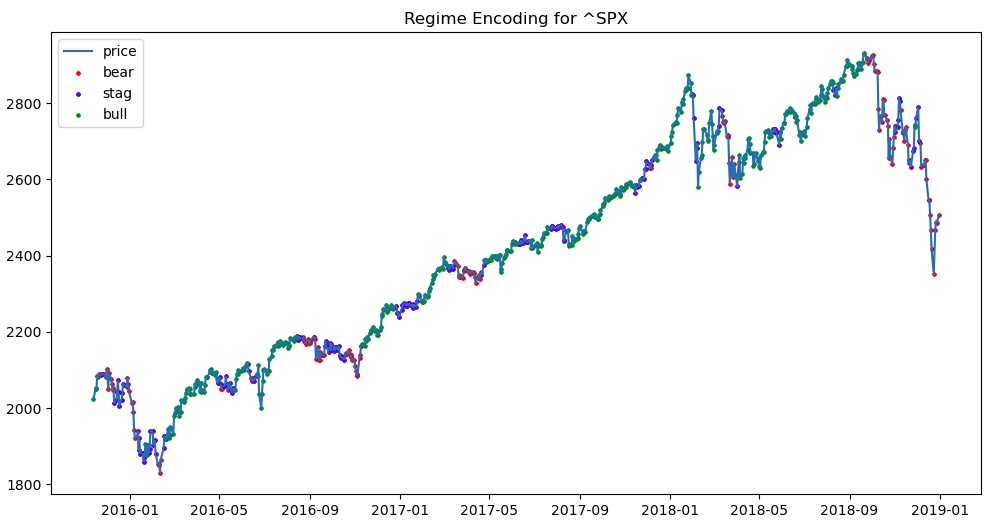
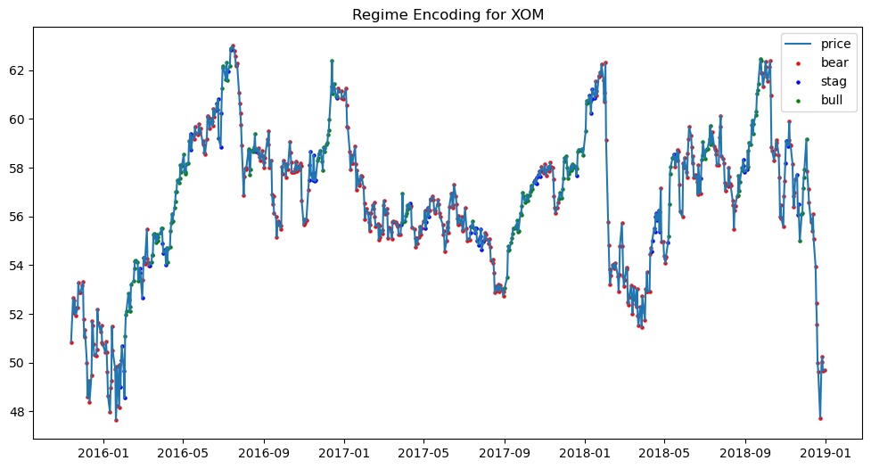
Figures 4.1 and 4.2 show two examples of HMM-encoded market regimes. The green dots represent periods where the HMM identified a bull market, red dots represent bear markets, and blue dots represent stagnant markets. In the case of ^SPX, the HMM appears to have identified upward trends as bull regimes and downward trends as bear regimes. With XOM, the encodings appear to be a lot messier: the HMM labelled many trends as bearish when they should probably be labelled stagnant or even bullish. Perhaps our assumptions about the distribution of price changes do not apply equally to all of our time series. We could probably build better HMMs by using different assumptions tailored to each feature, but this would come at the expense of being able to automate our model development process because we would need to manually identify regimes in order to identify their properties. Even with our suboptimal, automated approach to encoding market regimes, the Bayesian Network may still be able to accumulate enough information to make useful predictions. Let’s find out if that happens.
Structure Fitting
After encoding market regimes for our stock data, keeping the discretized target and economic data as-is, we will feed our CPCV training data into a Hill Climb Search algorithm. The Hill Climb is a heuristic approach to identifying Bayesian Network structures that explain the data. Heuristics are generally used where analytical solutions don’t exist and optimal solutions are computationally infeasible. We are looking for a directed acyclic graph (DAG) that connects all 22 feature-nodes, but the complexity of this kind of problem grows super-exponentially with the number of nodes. In other words, since we have no way to find the optimal solution, our next best bet is to find a good one. Using the pgmpy module, we can run a Hill Climb Search to fit a DAG structure that is good enough for our purposes.
To prevent the Hill Climb Search from consuming all available RAM and taking too long to process, we will limit the number of incoming edges for any node by setting max_indegree = 4. This results in a structure-fitting process that takes seconds rather than hours to complete.
Additionally, we will initialize the DAG with the following directed edges:
- ^SPX –> XLE, since the market probably influences the sector in a top-down fashion, like a tide influences a wave.
- PCU211211 –> CPIENGSL, since producer prices probably influence consumer prices
- IPN213111N –> CAPG211S, since drilling can be used to compute capacity
The Hill Climb Search may discard theses initial edges if it finds a better structure, but these will hopefully provide a helpful starting starting point for the algorithm. We will use the K2 scoring method to guide fitting algorithm, since that is what Alvi used in the original paper.
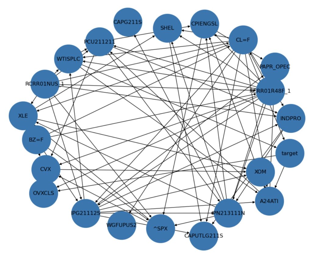
To visualize the resulting graph, we can use the networkxx module in combination with matplotlib. Figure 4.3 shows an example of one of the fitted DAGs. From this visual, we can see which features influence other features by noting the direction of the arrow on each connecting edge. While a node can have any number of outgoing edges (up to 21), each node can have at most four incoming edges.
Parameter Fitting
With our Bayesian Network’s structure established, we will then fit the parameters of the network to the data using the Bayesian Estimator from pgmpy with a K2 prior type. The core parameters of a Bayesian Network are conditional probability distributions (CPDs) that describe how each adjacent feature influences the other. Sometimes, the fitting process can result in nodes that have no CPD and this causes errors to occur during inference. To avoid that issue, we will provide uniform CPDs to any node that doesn’t yet have a CPD.
After fitting the parameters, we can then use the model for making predictions and evaluate the quality of those predictions using the metrics we defined in Step 1.
| Metric | Value |
|---|---|
| Accuracy | 0.699 |
| Precision | 0.704 |
| Recall | 0.711 |
| F1 Score | 0.708 |
| P(pred = 0) | 0.483 |
| P(pred = 1) | 0.517 |
| P(true = 0) | 0.488 |
| P(true = 1) | 0.512 |
| Metric | Value |
|---|---|
| Accuracy | 0.685 |
| Precision | 0.655 |
| Recall | 0.828 |
| F1 Score | 0.732 |
| P(pred = 0) | 0.344 |
| P(pred = 1) | 0.656 |
| P(true = 0) | 0.482 |
| P(true = 1) | 0.518 |
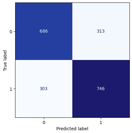
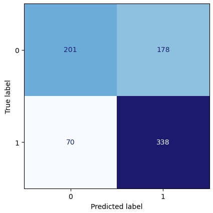
For this one CPCV train/val split, Figures 4.4 and 4.5 show the confusion matrices of our predictions and the true values. The values represent the number of points in each square; the colors give a visual indication of how those numbers compare to each other. We can see that, in the CPCV training set, the model made about twice as many correct predictions as incorrect predictions. In the CPCV validation set, the model was far better at catching positive price changes (1s) than negative price changes (0s).
Tables 4.4 and 4.5 show the key metrics, along with the distributions of predictions and true values. The model achieved 69.9% accuracy during CPCV training and 68.5% on the out-of-sample CPCV validation set. The model had a recall rate of 82.8% on the validation set, suggesting that it excelled at predicting price increases and missed relatively few of them. In both the CPCV training and CPCV validation sets, the true values were distributed roughly evenly (48%/52% split of 0s/1s). In the CPCV validation set, the model predicted 1s with 65.6% frequency, suggesting this model may be biased. Fortunately, with an accuracy of 68.5%, it is unlikely that the model’s success resulted purely from its bias. We will explore this thought process in more detail later.
Up until this point, we have been developing a single model using a single group from the CPCV combinations. Now we will use this same process to develop a model for every CPCV combination.
Step 5: Evaluate model development pipeline over entire CPCV set.
| accuracy | precision | recall | f1 | |
|---|---|---|---|---|
| count | 165 | 165 | 165 | 165 |
| mean | 0.685979 | 0.706053 | 0.672613 | 0.683045 |
| std | 0.019372 | 0.042091 | 0.094804 | 0.043233 |
| min | 0.623244 | 0.614657 | 0.408719 | 0.543919 |
| 25% | 0.673052 | 0.673378 | 0.614865 | 0.658885 |
| 50% | 0.689655 | 0.705215 | 0.678947 | 0.690860 |
| 75% | 0.698595 | 0.732394 | 0.733496 | 0.714628 |
| max | 0.729246 | 0.826923 | 0.925000 | 0.758910 |
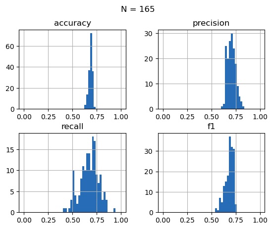
Running the model development process on each of the 165 combinatorial purged cross validation sets allows us to do more than just measure model performance — it allows us to determine the distributions of our performance metrics. This is because every time we measure the performance of a model, there is some uncertainty in our measurement. Random luck can cause the model to score better or worse on a given validation set, but taking many measurements allows us to characterize that uncertainty.
At first glance, these results look promising. The accuracy metrics are distributed around 68.6% with a standard deviation of 1.9%, suggesting the our HMM/BN approach is able to make correct predictions more often than not. Keep in mind that these accuracy measurements are for each model’s predictions on its respective CPCV Validation set after training on the CPCV Training set, so they are a decent estimate of out-of-sample performance. Now, let’s take a look at which features tend to appear most often in the Markov blanket for our target feature.
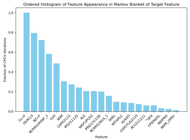
A Markov blanket is the set of nodes that provide information relevant for inferring a given node. Since we’re trying to predict the target variable, the Markov blanket includes parent nodes (features that directly impact the target), child nodes (features that the target directly impacts), and co-parent nodes (features that directly influence the same features that the target influences). All of these features provide information that is useful for inferring the value of the target.
With each CPCV iteration, we trained a new Bayesian Network with a new structure. By keeping track of which features appear in the target’s Markov blanket and how often, we can get a sense of which features tend to influence model predictions the most. Of all the features involved, CL=F, OVXCLS, BZ=F, RCRR01R48F_1, and CVX appear to have the largest impact on predictions. CL=F appears in 100% of the Markov blankets, which makes sense given that the target is simply the 5-day prediction for CL=F and that CL=F probably exhibits some degree of autocorrelation. On the flip side, PAPR_OPEC appears in only 1.2% of all the Bayesian Networks trained, suggesting it has limited usefulness in predicting oil price movements. We could probably drop most of these features from our search space without damaging our model development pipeline. This would allow us to increase the max in-degree to allow for more complex networks, or include other features not yet considered. For the purpose of this project, however, we will stick with the features we’ve got and see how well our approach handles the Validation set.
Step 6: Evaluate model development pipeline on Validation set.
Classification Metrics
Remember that we conducted CPCV within the Training set only. Using the exact same model development process, we can now train a model on the entire Training set and see how it performs on the Validation set, which no model has yet seen.
| Metric | Value |
|---|---|
| Accuracy | 0.698 |
| Precision | 0.723 |
| Recall | 0.780 |
| F1 Score | 0.750 |
| P(pred = 0) | 0.627 |
| P(pred = 1) | 0.373 |
| P(true = 0) | 0.581 |
| P(true = 1) | 0.419 |
The model predicted 0s in 62.7% of the cases, which parallels the fact that 58.1% of the true values were also 0s. Overall, this model achieved 69.8% accuracy — close to the expected 68.6% accuracy determine via CPCV. With the distribution of true values and predictions as they are, we would expect a model to achieve 52.1% accuracy if there were no underlying pattern in the market.
$$
\begin{align}
E(\text{accuracy})&=P(\text{pred=1} | \text{true=1}) + P(\text{pred=0} | \text{true=0}) \\
&=P(\text{pred=1}) * P(\text{true=1}) + P(\text{pred=0}) * P(\text{true=0}) \\
&=0.373 * 0.419 + 0.627 * 0.581 \\
&=0.521
\end{align}
$$
We can run the permutation test to see if our measured accuracy of 69.8% is significant.
Significance of Accuracy Measurement
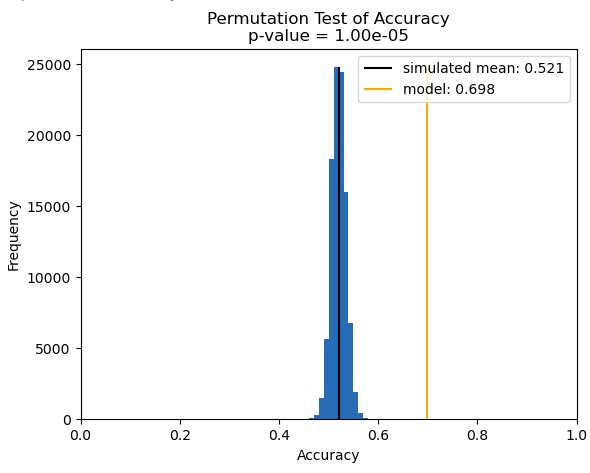
The permutation test shows that, in 100,000 worlds where market performance is truly random because no inherent structure exists, our model would have achieved accuracies between 45.0% and 58.3% with a median of 52.0% and a mean of 52.1% (as expected). In the real world, we achieved 69.8% accuracy. We can see from Figure 6.1 that the orange line, representing our measured accuracy, falls well outside of the distribution generated by permutation testing. With a p-value of 0.00001, the permutation test reveals a less than 1 in 100,000 chance that our model achieved this level of accuracy by chance, rather than by representing a legitimate structure in the market. That’s great news!
In order to build a profitable trading strategy, however, we need to balance our win rate (how often our hypotheses are correct) with our reward-to-risk ratio (how big of a dent we make on our P&L when we win compared to when we lose). But before we start simulating a trading strategy, we can learn a lot about reward and risk by looking at the distribution of returns conditioned on our model’s predictions.
Distribution of True Returns Conditioned on Predictions
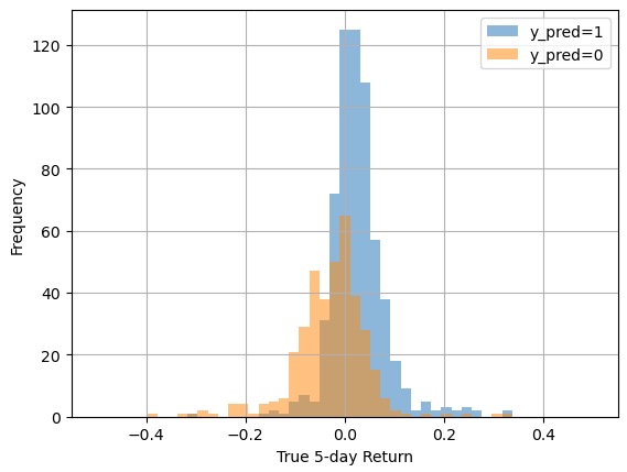
returns for each predicted class.
| Pred = 1 | Pred = 0 | |
|---|---|---|
| mean return | 0.021713 | -0.029461 |
| mean log return | 0.025184 | -0.033103 |
| sum log returns: correct | 21.875441 | -17.166395 |
| sum log returns: incorrect | -6.009668 | 4.719649 |
| net log return | 15.865773 | -12.446746 |
predicted class in the Validation set.
As hoped, the times when the model predicts positive price changes have a mean return of +2.2% (including the times when the model is wrong); likewise, the times when the model predicts negative price changes have a mean return of -2.9%. In other words, the model is providing a signal that could probably support a profitable trading strategy. To see if that is true in aggregate, we will use logarithms to transform our returns into log returns, which can be added up over time (as opposed to regular returns which must be summed with 1.0 and then multiplied). The “mean log return” accounts for the compounding nature of returns and confirms what the arithmetic mean reveals.
If we consider the sum of log returns whenever the model makes a correct prediction and compare that to the sum of log returns whenever the model’s prediction is wrong, we can determine whether the net log return is agreeable. As we can see from our data table, the model has a net log return of +1587% for positive predictions over the four years from Jan 2019 to the end of 2022, while the model has a net log return of -1245% for negative predictions. These net log returns include all the cases where the model predictions were wrong. That’s a great sign: we want the true returns to be cumulatively negative whenever the model predicts a “0” (a price decline) and we want the true returns to be cumulatively positive whenever the model predicts a “1”.
During computation of the log returns, numpy threw a RuntimeWarning telling us there was an invalid value. This often occurs because of negative values, for which logarithms are undefined. Let’s take a look at all the cases in our validation set where the 5-day returns might have been worse than -100%:
- 2020-04-20, target = -2.679161
- 2020-04-27, target = -1.339623
We can now see exactly when the target variable experienced such a large negative return that \(\log(1 + r)\) threw a warning: once on the infamous April 20, 2020, when oil prices went negative because COVID caused people to stop driving and oil storage costs were priced higher than the value of the oil itself; and once more on April 27 — exactly five trading days later — because even though the absolute return was positive, the percent return was negative due to the negative entry price on April 20. This exceptional market event posed a massive risk to anyone who was fully invested or worse, overleveraged, in oil during that time. Without derivative instruments, the only way to mitigate that kind of risk in the future is to not allocate too large a fraction of one’s portfolio on any single trade or instrument. That said, for the purposes of testing our model in a trading strategy, we will allow full allocation.
Step 7: Evaluate model performance by proxy: model-informed strategy performance on Test set.
Since our primary goal here is to demonstrate the usefulness of HMM-encoded regimes and Bayesian Networks, we won’t spend too much time developing a robust trading strategy or strategy development framework. Instead, we will train a model using the same process as before, but this time on the combined Train-Val sets. We will then retrieve the model’s predictions over the entire Test set and simulate the realized profit-and-loss for two strategies: a simple long-only strategy and a long-short strategy.
The rules for the long-only strategy are as follows:
- If model predicts a price increase, go long with a 20% allocation of portfolio funds (since the prediction horizon is 5 days, so we can have up to 5 concurrently open trades). Exit positions at the close of the fifth day.
- If the model predicts a price decrease, do nothing. Do not close open positions; do not open new positions.
The rules for the long-short strategy are as follows:
- If model predicts a price increase, go long with a 20% allocation of portfolio funds. Exit positions at the close of the fifth day.
- If the model predicts a price decrease, go short with a 20% allocation of portfolio funds. Exit positions at the close of the fifth day. Note that, while brokers may follow FIFO logic for individual accounts, traders and firms in the USA are legally permitted to manage opposing trades on the same instrument in different accounts for legitimate trading purposes.
We will model trading fees, slippage, and margin interest, as a bundled per-trade expense. As of September 1st, 2025, Schwab’s pricing table shows a 2.25 USD per-contract fee for futures while Yahoo Finance lists CL=F at 64.92 USD per barrel for contracts of 1000 barrels each, so the 4.50 USD round-trip trading fee on a single 64,920 USD contract represents 0.007%. Combine that with Schwab’s ~12% annualized margin interest rate over the 5 days each position will remain open, we arrive at fees representing 0.17% of each trade (Schwab’s 2.25 USD trading fee is neglible). Tack on +/- 5 cents of average slippage on each trade for a total 0.25%. We will round this up to 0.3% per trade to be on the safe side.
$$\text{Trading Fees} + \text{ Margin Interest} + \text{ Slippage} = \frac{4.50}{64920} + 5 * \frac{0.12}{360} + \frac{0.05}{64.92} = 0.0025 \approx 0.3\% \text{ per trade}$$
For simplicity, we will allow fractional positions in all strategies. We will not model stop orders, unrealized P&L due to intraday price action, or margin maintenance requirements. Concurrent long and short positions are allowed, because traders or firms may manage long/short positions on the same instrument in separate accounts.
Classification Metrics and Significance
| Metric | Value |
|---|---|
| Accuracy | 0.672 |
| Precision | 0.702 |
| Recall | 0.616 |
| F1 Score | 0.656 |
| P(pred = 0) | 0.446 |
| P(pred = 1) | 0.554 |
| P(true = 0) | 0.509 |
| P(true = 1) | 0.491 |
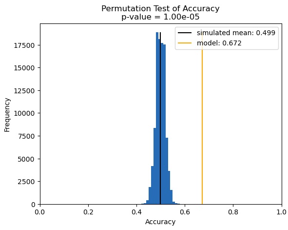
The final model, trained on Train + Val and evaluated on Test, achieved 67.2% prediction accuracy with a 55%/45% split of 1s/0s predicted. The true values had a 49%/51% split of 1s/0s. The permutation tests confirmed statistical significance to the 0.00001 level.
Distribution of Returns Conditioned on Predictions
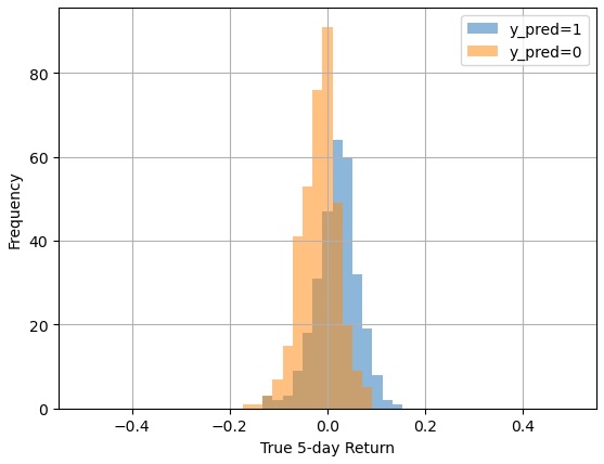
returns for each predicted class.
| Pred = 1 | Pred = 0 | |
|---|---|---|
| mean return | 0.019085 | -0.016461 |
| mean log return | 0.017971 | -0.017414 |
| sum log returns: correct | 8.337296 | -9.442161 |
| sum log returns: incorrect | -2.964041 | 2.981516 |
| net log return | 5.373255 | -6.460644 |
predicted class in the Test set.
So far, our Test set seems to be confirming what we saw in the Validation set: a strong out-of-sample performance. With 1.9% mean returns for predicted price increases and -1.6% mean returns for predicted price decreases, the model is generally achieving good results. The ultimate test is whether these good classification results translate into good trading outcomes.
Backtesting Long-Only and Long-Short Strategies Guided by Model’s Predictions
Earlier on, we defined the metrics we want to apply to each trading strategy. Some of those metrics require an annualized risk-free rate, so we will import the 4-week treasury bill secondary market rate (“DTB4WK”) from the FRED API for that purpose. We will make sure it is sorted chronologically, then forward fill any missing values. We will select only those rates applicable to the Test set timeline and, since FRED returns these values as percentages, we will divide by 100 to convert them to ratios.
When computing returns, we will apply our 0.3% fee to each return regardless of outcome, and make sure to allocate only 20% of the portfolio to each concurrent trade. The baseline buy-and-hold strategy will allocate 100% on its one and only trade. Altogether, we will test three different strategies, feeding n=3 into the function that computes the Deflated Sharpe Ratio.
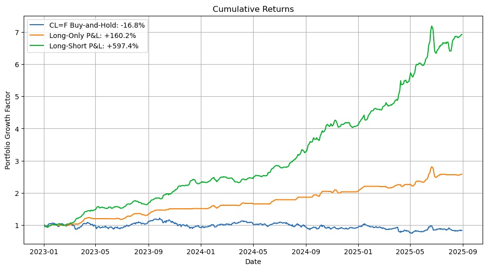
| Strategy | Final P&L | Max Drawdown | Calmar Ratio | Omega Ratio | Sharpe Ratio | Probabilistic Sharpe Ratio | Deflated Sharpe Ratio |
|---|---|---|---|---|---|---|---|
| Buy-and-Hold | -16.8% | -39.0% | -0.3 | 1.0 | -0.2 | 0.5 | 0.01 |
| Long-Only | 160.2% | -11.8% | 3.2 | 2.2 | 3.3 | 1.0 | 1.0 |
| Long-Short | 597.4% | -11.8% | 8.6 | 2.4 | 5.3 | 1.0 | 1.0 |
Between Jan 2023 and Sept 2025, the buy-and-hold strategy on WTI Oil Futures (where we roll the position at the end of each month when contracts expire) would have lost 16.8%, but the model-informed long-only and long-short strategies would have gained 160% and 598%, respectively. Not only did our model produce higher returns, it also reduced the max drawdown from 39.0% down to 11.8% — to less than a third. With comparatively high Calmar and Omega ratios and large, positive Sharpe ratios (in contrast to the baseline’s negative Sharpe), both model-informed strategies far exceeded the market’s performance. The high Probabilistic and Deflated Sharpe Ratios indicate that our true Sharpe ratios are in the near-100th percentile of what can be produced by the benchmark strategy or by noise. In other words, we beat the benchmark decisively.
Summary
We explored how to use Hidden Markov Model’s to encode stock market regimes and how to use Bayesian Networks to predict price movements for oil futures five days in advance. In the process, we:
- Took macro-economic and stock market data from the Yahoo Finance, FRED, and EIA databases, computed percent changes for each series, and shifted each series forward to appropriately capture the lag between the period each data point represents and the time when data becomes available for use in trading.
- Split the data into Train, Validation, and Test sets, performed Combinatorial Purged Cross Validation within the Train set to identify a promising model development process, evaluated that process on the out-of-sample Validation set, and concluded that our process was worth testing in a paper trade simulation.
- Re-ran the model development process from scratch on the combined Train + Validation sets, and then evaluated the model’s performance on the out-of-sample Test set by computing classification metrics (accuracy, precision, recall, f1-score), examining the conditional distributions of true returns given the model’s predictions, conducting a permutation test, and comparing the portfolio metrics of two different trading strategies against a baseline buy-and-hold strategy.
Our model provided a statistically significant trading signal that gave two basic strategies enough “edge” to drastically outperform the benchmark from 2023 to late 2025, deploying one-fifth of the portfolio per trade. In the end, these results demonstrated the potential for HMM-informed Bayesian Networks to identify true patterns in oil markets.
Future analyses could explore:
- Using different features.
- Shorter prediction horizons.
- Alternative target instruments (like BZ=F).
- Bayesian Networks with higher limits on in-degree.
- Different commodities markets, like metals or crops.
- Different securities markets like stocks or volatility swaps.
- Discretizing by percentile rather than binary discretization.
- Kernel density estimated conditional probability distributions rather than discrete tables.
- Methods for improving HMM regime detection, such as continuous emissions or tailored assumptions.